This page benchmarks the implementation of a speech-to-text solution on a Xilinx edge device using the Vitis accelerated flow. The model chosen for the automatic speech recognition (ASR) task is Baidu’s DeepSpeech2. Results are broadly discussed for three designs, two designs run only on the processing system (PS) and the third design offloads some computation on the programmable logic (PL) in combination with the PS. The designs are evaluated on Zynq UltraScale+ MPSoC ZCU102 evaluation kit and the comparative results are reported.

Table of Contents

Introduction

Machine learning (ML) and deep learning (DL) based solutions have become the new normal. Be it an image, video, speech or text, all forms of data are being processed by ML/DL solutions and utilized for a variety of applications. The area of speech and language processing, categorized as Natural Language Processing (NLP), is an active area where ML/DL is being applied to provide new ASR solutions.  Generally, most solutions are compute-intensive and require high-end graphics processing units (GPUs) or cloud-based inference. However, GPUs are power hungry and cloud-based solutions raise  questions about privacy and data security. Field Programmable Gate Arrays (FPGAs) solutions have evolved to include the combination of Processor Subsystems combined with traditional FPGA logic, enabling power efficient, edge-base solutions for these traditionally compute-intensive tasks. Due to these advantages, there has been a trend to target more and more complex ML/DL solutions on edge-based FPGA system-on-chip (SoC) devices.

This page benchmarks a pre-recorded audio file-based standalone speech-to-text translation application, on a Xilinx SoC device, using the Vitis Unified Software Platform acceleration flow.

Speech-to-Text Translation

A speech recognition task involves three major steps, as shown in the below figure. It shows a top-level diagram for a speech-to-text conversion task.

The three major blocks are:

1. Feature Extraction:  Given an input audio file, it is required to extract the information in a form which can be interpreted by a deep learning model. This information extraction step is termed as a feature extraction step. For a speech recognition task, a spectrogram is generated from the audio file and it is given as an input to the deep learning model.

2. Deep Learning Model: A trained deep learning (DL) model receives input from the feature extraction block and predicts the output. For speech recognition tasks the DL models are generally based on a Long Short-Term Memory (LSTM) model.

3. Decoder: The output of the DL model are numbers/probabilities which need to be interpreted as the final prediction. The Decoder performs this task and it is generally based on a CTC (Connectionist Temporal Classification) decoder. The decoder finally predicts the equivalent text of the input audio.

The NLP task of speech-to-text translation is a compute-intensive task, and this page aims to benchmark this algorithm implementation on the Xilinx Zynq UltraScale+ series of SoC.  The Zynq UltraScale+ family features a heterogeneous processing system comprised of a low-power 64bit quad-core ARM Cortex-A53 processing unit running up to 1.5GHz, supporting advanced SIMD, VFPv4 floating-point extension instructions.  The aim is to benchmark this type of task on the Zynq UltraScale+ as an exercise to demonstrate the relationship between the algorithm compute requirements and hardware solutions to support standalone edge-based implementations.

Brief Overview of DeepSpeech2

Baidu's DeepSpeech2 is an end-to-end solution for automatic speech recognition (ASR). The model intakes normalized sound spectrogram as an input (generated by feature extraction step) and generates a sequence of characters, which are then reduced to final prediction by a decoder. The general architecture of the DeepSpeech2 model is shown by the left image in the figure below. The number of CNN and RNN layers can vary as mentioned in the DeepSpeech2 paper.

The model intakes a normalized spectrogram. The input is then passed through a set of convolutional (CNN) layers. After the convolutional layers, there is a stack of LSTM layers (it can be a simple Recurrent Neural Network (RNN) , or Gated Recurrent Unit (GRU) also). These LSTM layers are generally bi-directional layers, which process frames in both forward and backward directions. The LSTM layers are then followed by a fully connected (FC) layer. The output of the FC layer is then passed to a CTC-based decoder to predict the final text output.

Architecture of DeepSpeech2 Model used for Benchmarking

The architecture used is shown on the right side of the figure above. The model implemented consists of a stack of bi-directional LSTM layers along with other layers such as CNN and FC. The implementation is a dense model (not pruned) that is deployed without quantization and leverages a 2-layer CNN and a 5-layer bi-directional LSTM. The numbers mentioned in the figure correspond to a convolutional layer representing input channels, output channels, filter height, filter width, stride height, and stride width respectively. The input size and the number of hidden units in each gate are also mentioned for all the LSTM layers (input size, number of hidden units).

LSTM cell overview

The LSTM cell used by the DeepSpeech2 model is shown in the below figure. It is a standard LSTM cell with no “peephole” connections (i.e. the gate layers do not read the cell states) as represented by the set of equations in the figure. Depending on the input audio length the LSTM cell calculates the output for a fixed number of timesteps. At every timestep ‘t’, these equations are to be computed, where ‘W’ represents a weight matrix, ‘b’ represents the biases, ‘x’ is the input vector to the LSTM cell and ‘y’ is the output vector of the LSTM cell.

For every timestep ‘t’, input vector corresponding to the same time step ‘x_t’ is multiplied by a weight matrix, while output vector ‘y_t-1’ of previous time step is multiplied by a weight matrix. Thus, there is a feedback between every timestep, which is one of the bottlenecks in achieving maximum parallelization of an RNN based model.

For one LSTM cell, ‘i_t’, ‘f_t', ‘o_t' and ‘g_t' represent the four major gates (input gate, forget gate, output gate and intermediate cell gate respectively).

Every gate has two weight matrices (’W_{_x}'and ‘W_{_r}') and a bias term (’b_’) associated to it (e.g. ‘W_ix', ‘W_ir' and ‘b_i' for input gate). The ‘W_{_x}' matrix is multiplied with the input vector ‘x_t' and the 'W_{_r}' matrix is multiplied with the recurrent output vector of previous time step 'y_t-1'. Every gate output is the result of a nonlinear function (sigmoid or tanh) applied to the summation of the two matrix-vector products and the bias term. Finally the gate outputs ( ‘i_t’, ‘f_t', ‘o_t' and ‘g_t') and the previous cell state (’c_t-1’) are used to obtain the new cell state (’c_t’) and the output of LSTM cell (’y_t’).

This Wiki page provides a comparison result of two implementations, one which runs only on the PS and other which uses both PS and PL. The application is tested on a ZCU102 board, which reads an audio file from the SD card and prints the predicted text on the screen.

Specific Details of Implementation

Hardware and Software requirements

The hardware and software resources used for the implementation:

• Xilinx ZCU102 evaluation kit

• USB type-A to USB mini-B cables (for UART communication)

• Secure Digital (SD) memory card

• Xilinx Vitis 2019.2

• Xilinx Vivado 2019.2

• Xilinx Petalinux 2019.2

• Serial communication terminal software (such as Tera Term or PuTTY)

Details of DeepSpeech2 model used

The DeepSpeech2 model used for benchmarking the two designs:

• Model Size: ~196 MB

• Precision: Single Precision Floating Point (32-bit)

• Pruning: No

• Quantization: No

• Training Dataset: LibriSpeech dataset

• Word Error Rate (WER): 10.347 (on ‘test_clean’ subset of Librispeech)

 Details of Input Audio File

• File Format: Wav file

• Format: PCM

• Format settings:

  • Endianness: Little

  • Sign: Signed

• Codec ID: 1

• Bit rate mode: Constant

• Bit rate: 256 Kbps

• Channel(s): 1 channel

• Sampling rate: 16.0 KHz

• Bit depth: 16 bits

Designs Implemented

We benchmark broadly two designs, one which runs only on the processing system (PS only) and other which runs on a combination of processing system and programmable logic (PS+PL).

PS only solution

The complete DeepSpeech2 pipeline is implemented using C++. The complete pipeline is developed in-house from scratch and no external high-end libraries or IP cores are used. The design is compiled and built using the Vitis acceleration flow and then tested on ZCU102 board using the executables generated by Vitis. The initial version of the implementation was profiled for 10 audio samples, with the samples ranging from 1 second to 11 seconds. The profiling results are shown in the table below.

Profiling the pipeline resulted in the following major takeaways: 

1. The time taken for the initial PS only solution computing the complete pipeline was on an average equal to 6.77 times the audio length.

2. The combined time taken by feature extraction and post LSTM block is less than 1% of the total time taken.

3. On average, the time spent in computation of the CNN block is around 11% for all the audio samples.

4. As expected, the LSTM block is the most expensive block and consumes around 89% of the total computation time.

After profiling the initial PS-only solution, to achieve better performance  a multi-threaded design is then implemented to reduce the computation time and utilize the ARM cores efficiently.

Optimized Multi-threaded PS only solution

The initial PS-only solution is modified using a multi-threaded approach to make use of the four ARM cores available. The CNN block and LSTM block computations are parallelized using four threads and helped to bring down the computation time. Table below shows the profiling numbers for the optimized PS-only solution.

Key observations after profiling the multi-threaded PS-only solution are as follows:

1. The multi-threaded implementation of CNN and LSTM blocks helped in considerably reducing the overall run time.

2. Overall run time reduced from the initial 6.77 times to 1.887 times the audio length. This amounts to approximately 72% reduction in the run time.

3. The CNN block now contributes to around 12% of the total run time.

4. Still, the LSTM block is the major block in terms of computation time and consumes around 87% of the total computation time. 

The next step is to offload some of the computations into the programmable logic (PL) and try to achieve more acceleration. As LSTM block is the major time-consuming block, so is the ideal candidate for being accelerated in PL.

PS +PL solution

The LSTM block mainly consists of computing the equations mentioned in the figure in LSTM cell sub section. The major time-consuming operation in these equations is the matrix-vector multiplication for every gate (‘Wx’ and ‘Wy’).

As explained previously, for ‘Wx’ computation, ‘x’ is the input of current timestep (‘t’) and there is no dependency on the previous time step, thus it is termed a non-recurrent computation. While for ‘Wy’ computation, the vector ‘y’ is the output of the previous timestep (t-1), thus a feedback and  the ‘Wy’ computation is termed a recurrent computation. In the PS+PL design, the ‘Wx’ computation is accelerated in the PL. The matrix-vector multiplication is converted into matrix-matrix multiplication, by bringing the ‘Wx’ computation outside of the non-linear functions. Tiling, pipelining and unrolling are carried out to accelerate the matrix-matrix multiplication on PL. An option of also accelerating ‘Wy’ computation in PL was explored, but was not achievable due to two bottlenecks: the feedback nature of the computations, and  the limited on-chip memory available on the Zynq UltraScale+ device on the ZCU102 board. Thus, only ‘Wx’ computation of all LSTM cells (for both forward and backward pass) is accelerated on the FPGA fabric and rest all computations of the pipeline are carried out on the ARM cores (similar to the multi-threaded PS only solution).

 The design is synthesized for an operating frequency of 200MHz. The resource utilization summary of the PS+PL design is shown in the below table. Apart from Block RAM (BRAM), other resources used are relatively low.

Figure below shows the top-level block diagram of the PS+PL implementation. The audio file is read from the SD card. Then feature extraction and CNN are processed  on the PS, after which the LSTM block is executed using both PS and PL. The remainder of the pipeline is again executed on PS, and finally the predicted text is printed on a terminal using UART. External DDR memory is used to store the model weights and the intermediate results. These weights are fetched from DDR and stored locally in the on-chip BRAM.

The PS+PL design is also profiled for the same ten audio samples and the results are shown in the table below.

The following points are derived from the profiling data: 

1. As expected, the time taken by feature extraction, CNN and post-LSTM blocks remain the same for both PS-only (4 threads) and PS+PL solutions.

2. There is approximately a 40% speedup in the processing time for LSTM blocks after ‘Wx’ computation is accelerated using PL resources.

3. The overall time taken by the complete pipeline is reduced to around 1.247 times  the input audio length.

4. Compared to PS-only (4 threads) there is a reduction of around 36% in the computation time.

Results Comparison

In this section we compare the runtime achieved by the three designs for all the 10 audio samples.

Table below compares the total runtime of the three designs, and PS+PL is the fastest.

Figure below displays the normalized runtime for each of the separate processing blocks of the pipeline. The runtime is normalized with respect to the input audio length. The best runtime of 1.247x is provided by the PS+PL solution.

How to Run the Demo using Binaries

NOTE: Contact Xilinx Technical Marketing team for binaries.

The top level contents of the zip are as shown in the figure:

Sample Audios for testing the demo are in the “audios” folder and the model weights are present in the “weights” folder. Three executables (“STT_PS.exe”, “STT_PS_NoThreads.exe” and “STT_PSPL_200MHz.exe”) for the three designs are there along with the “BOOT.bin” and “image.ub”. The xclbin file “matmul.xclbin” which is required by the “STT_PSPL_200MHz.exe? is also present.

Steps to setup the demo:

• Extract the zip and copy the contents in a SD card. 

• Insert the SD card on ZCU102 board.

• Make sure the board is set to SD card boot mode (follow page 21, table 2-4 in user guide).

• Connect Power cable and the UART cable.

• Power ON the board.

• Open and setup up Putty/Tera Term (or any other terminal emulator) in your machine/laptop with a baud rate of '115200' (This link can be useful). 

• You should see a prompt root@xilinx-zcu102-2019_2:~#

• Set the XRT enviornment variable using: export XILINX_XRT=/usr

• Now mount the SD card using the command: mount /dev/mmcblk0p1 /mnt/

• Enter the /mnt folder using command: cd /mnt

• Run the command “ls” you should be able to see the SD card contents now.

PS only (no threads)

• Run the application with the path of the audio passed as an argument. 

  • Ex. to convert audio file 1SEC_1.wav run the command

    • ./STT_PS_No_Threads.exe

    • Enter audio file name: audios/1SEC_1.wav

• The predicted text and the time taken will be printed as an output on the terminal as shown below.

PS Only (Multithreaded)

• Run the application with the path of the audio passed as an argument. 

  • Ex. to convert audio file 1SEC_1.wav run the command

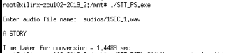
    • ./STT_PS.exe

    • Enter audio file name: audios/1SEC_1.wav

• The predicted text and the time taken will be printed as an output on the terminal.

PS+PL

• Run the application with the path of the audio passed as an argument.

  • Ex. to convert audio file 1SEC_1.wav run the command

    • ./STT_PSPL_200MHz.exe matmul.xclbin

    • Enter audio file name: audios/1SEC_1.wav

• The predicted text and the time taken will be printed as an output on the terminal.

NOTE: Due to context switching, for different runs there will be minor variation (3rd decimal place) in the time taken for conversion.